Census Data

import geopandas as gpd
from matplotlib import pyplot as plt
from tobler.area_weighted import area_interpolate
import hvplot.pandas
import geoviews.tile_sources as gvts

# import previous variables utilized in this analysis

# original elementary catchment areas 
school_ct_es = gpd.read_file('./data/psd_catchments/SchoolDist_Catchments_ES.geojson').to_crs(3857)

# filtered catchment areas
school_ct_es_filt = gpd.read_file('./data/psd_catchments_filtered/catchments_filt_elementary.geojson', driver='GeoJSON')
school_ct_ms_filt = gpd.read_file('./data/psd_catchments_filtered/catchments_filt_middle.geojson', driver='GeoJSON')
school_ct_hs_filt = gpd.read_file('./data/psd_catchments_filtered/catchments_filt_high.geojson', driver='GeoJSON')

Census Data Analysis

Demographic characteristics at the catchment level can be utilized to understand the general composition of the neighborhoods that each school serves. The Census Bureau does not publish statistics at this geography, but through a method called Areal Interpolation, demographic variable values derived at the census tract level can be distributed for each catchment zone to get a reasonable estimate.

Census data was acquired from the ACS 5-Year estimates for the year 2023. Variables pulled in this analysis and their associated table codes were: - Total Tract Population (B01003) - Population in School (B14001) - Population in an Undergraduate Program (B14001) - Population in a Graduate Program (B14001) - Population Not in School (B14001) - Total Households (B11001) - Family Households (B11001)

Total Tract Population will be utilized to calculate the population density of each tract, which serves as an indication of how efficiently a new SRTS project would serve the community. Denser tracts will be able to utilize SRTS infrastructure much more readily than tracts with lower population densities. Similarly, the proportion of students are enrolled in a K-12 program within a district (calculated from the difference between the total population in School and the total populations in an Undergraduate/Graduate program or are Not in School) serves as an indicator of demand for SRTS projects. Finally, since families with toddler-aged children that are not presently in school aren’t reflected in this measure, the proportion of family households within a tract is also calculated.

# read in census data from file
acs_data = gpd.read_file('./data/phl_acs2023_tracts.geojson')

# plot census track geometries and elementary catchment zone geometries overlapped to compare boundaries
ax = acs_data.plot(figsize=(8,8), color='lightgrey', edgecolor='white', alpha=1)
school_ct_es.to_crs(3857).plot(ax=ax, color='none', edgecolor='red', linewidth=1).set_axis_off()
plt.title('Philadelphia Census Tracts (grey) and\nElementary School Catchment Areas (red)', fontsize=14)
plt.show()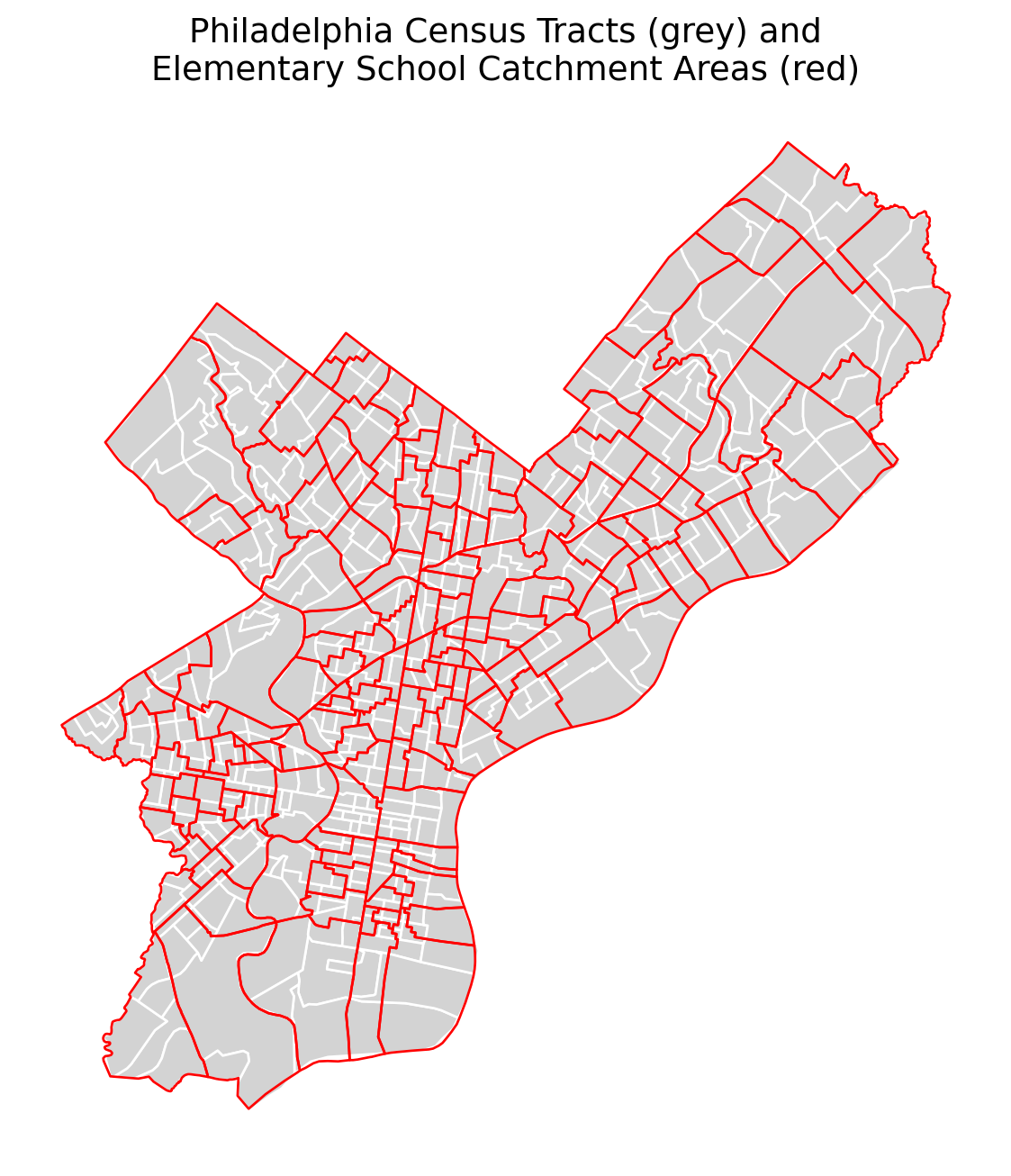

Census tract boundaries do not like up perfectly at all with scchool catchment zones. In order to assess the average census characteristics within each catchment area, we need to areal interpolate these values. This involves using the percent overlapping area between the source (census tract) and target (catchment area) to portion out the total value within a census tract. These “chunks” of value are summed within each catchment area to get an estimated total value for that area. This process is repeated for each variable of interest, and will be repeated for each catchment area type (elementary, middle, high). This method distinguishes between extensive and intensive variables - extensive variables are those that are additive in nature (i.e. total population), while intensive variables are ratios or percentages (i.e. percent of population below poverty line). Extensive variables can be summed directly, while intensive variables need to be recalculated after the interpolation process.

acs_data.columns

Index(['GEOID', 'pop', 'in-sch', 'in-undgrd', 'in-grd', 'not-in-sch',
       'tot_hhds', 'fam-hhds', 'state', 'county', 'tract', 'NAME', 'pop_moe',
       'in-sch_moe', 'in-undgrd_moe', 'in-grd_moe', 'not-in-sch_moe',
       'tot_hhds_moe', 'fam-hhds_moe', 'geometry'],
      dtype='object')

ext_vars = ['pop', 'in-sch', 'in-undgrd', 'in-grd', 'not-in-sch', 'tot_hhds', 'fam-hhds']

# areal interpolation of census data to elementary school catchment areas using the tobler library
acs_es = area_interpolate(
    source_df=acs_data,
    target_df=school_ct_es_filt,
    extensive_variables=ext_vars
)

# interpolate middle school catchment areas
acs_ms = area_interpolate(
    source_df=acs_data,
    target_df=school_ct_ms_filt,
    extensive_variables=ext_vars
)

# interpolate high school catchment areas
acs_hs = area_interpolate(
    source_df=acs_data,
    target_df=school_ct_hs_filt,
    extensive_variables=ext_vars
)

# plot hvplot of census tract population before interpolation
tract_pop_plot = acs_data.hvplot(
    color='pop',
    geo=True,
    title='Census Tract Population Before Interpolation',
    crs=3857,
    cmap='reds',
    height=600,
    width=600
)

gvts.CartoLight * tract_pop_plot

# plot hvplot of elementary school catchment area population after interpolation
es_pop_plot = acs_es.hvplot.polygons(
    color='pop',
    geo=True,
    title='Elementary School Catchment Area Population After Interpolation',
    crs=3857,
    cmap='reds',
    height=600,
    width=600
)
gvts.CartoLight * es_pop_plot

Note that some population patterns are revealed more clearly when aggregated to the catchment level, with a significant density of population in Center City. Similarly, some areas of South Philadelphia that originally seemed to have higher population counts compared to the rest of the city at the tract level fall behind other catchment areas elsewhere in the city when aggregated to the catchment level. Missing tracts due to a lack of associated school point also become apparent here, but their absence does not impact the results of interpolation.

# join all sets of interpolated data to filtered school catchments gdfs to link IDs
acs_es_schools = school_ct_es_filt[['ES_ID', 'geometry']].join(acs_es.drop(columns='geometry'))
acs_ms_schools = school_ct_ms_filt[['MS_ID', 'geometry']].join(acs_ms.drop(columns='geometry'))
acs_hs_schools = school_ct_hs_filt[['HS_ID', 'geometry']].join(acs_hs.drop(columns='geometry'))

These variables will be min-max normalized in order to accurately represent the fluctations in demographic variables over the region.

# define function to calculate specified demographic metrics and index values
def add_acs_calculations(df):
    df = df.copy()
    
    # compute area in square miles
    df['area_sqmi'] = df.geometry.area / 2589988.11034
    
    # derive percent and normalized count metrics
    df = df.assign(
        in_sch_pct = df['in-sch'] / df['pop'],
        fam_hhds_pct = df['fam-hhds'] / df['tot_hhds'],
        pop_dens = df['pop'] / df['area_sqmi']
    )
    # create a normalized index value for each column
    df['in_sch_idx'] = (df['in_sch_pct'] - df['in_sch_pct'].min()) / (df['in_sch_pct'].max() - df['in_sch_pct'].min())
    df['fam_hhds_idx'] = (df['fam_hhds_pct'] - df['fam_hhds_pct'].min()) / (df['fam_hhds_pct'].max() - df['fam_hhds_pct'].min())
    df['pop_dens_idx'] = (df['pop_dens'] - df['pop_dens'].min()) / (df['pop_dens'].max() - df['pop_dens'].min())

    return df

# calculate 
es_schools_calc = add_acs_calculations(acs_es_schools)
ms_schools_calc = add_acs_calculations(acs_ms_schools)
hs_schools_calc = add_acs_calculations(acs_hs_schools)

# isolate index columns
idx_cols = ['in_sch_idx', 'fam_hhds_idx', 'pop_dens_idx']

# sum the catchment-area-based demographic index value based on specified columns 
def calc_index(df, id_col):
    df_select = df[[id_col, 'geometry'] + idx_cols].copy()
    df_select['demo_index'] = df_select[idx_cols].sum(axis=1)
    return df_select

# calculate index values for all levels of school catchment area
es_index = calc_index(es_schools_calc, 'ES_ID')
ms_index = calc_index(ms_schools_calc, 'MS_ID')
hs_index = calc_index(hs_schools_calc, 'HS_ID')